
Open Source Superconducting Circuit Design
Messing around with scqubits and SQcircuit

This is Part I of an indefinitely long series on superconducting circuit design using open software. I’ll update this section with links to the following installments when they’re available.
Also you can find the code I used to make the plots at my GitHub repo.
EDIT: Forgot to welcome the many new subscribers, we now number > 100. I am not sure what you thought you were signing up for, but I hope you enjoy the ride.
Now that there are at least two open-source superconducting circuit simulators, scQubits and SQcircuit, I’ve started wondering how easy it would be for someone to do a non-trivial circuit design using only open-source software. That means going from the concept and initial Hamiltonian solving, through physical simulation, and culminating in circuit layout. Realistically this would be an iterative process as you learn more about the trade-offs you’ll have to make to realize a working, testable device. This endeavor should also force me to actually learn more about these softwares beyond the fact that they exist.
Our Goal
We will seek to recreate Google’s quantum supremacy architecture1 (Sycamore), so we’ll simulate two of their transmons coupled together with one of their couplers. Since every element is tunable, we can showcase the flux biasing functionality of the simulators, plus Google’s choice of coupler minimizes the number of nodes in our simulation, so I think it should be tractable even on a laptop. If you have access to some high-performance computing (HPC) resources, you can then generalize this to more complicated circuits with more nodes.

Step 1 (this post) is going to be solving for the eigenspectrum of a coupled 2-qubit system to figure out what circuit parameters we’ll need to hit our frequency and coupling targets.
Subsequently, we’ll guess some reasonable fabrication design rules and actually draw our structures, export them to a physical simulator and see what changes we need to make to hit our circuit parameter targets. That’ll probably be a separate post.
The Humble Transmon
We’ll start by defining our simple transmon qubit, the workhorse of superconducting quantum computing (as of early 2022). Recall from a previous post that we prefer qubits with frequencies between 4-8 GHz. Let’s choose 6 GHz. What other parameters do we need to specify? We also need to specify the anharmonicity, α. That will tell us the difference between the energies of the first and second excited states (in GHz), and it also puts a speed limit on how fast we can excite our qubits with microwave pulses2. Let’s choose -200 MHz.
Ok so. How do we figure out the circuit parameters? Let’s pull up the original transmon paper and take a look at the expression for eigenenergies:

Some definitions:
m is the index of the eigenstate. m = 0 would be the ground state, m = 1 is the first excited state, etc.
Ej is the Josephson energy.
Ec is the charging energy of the capacitor.
Em is the energy of the mth eigenstate.
We are going to set m = 1, so that the energy is 6 h*GHz, where h is Planck’s constant. You’ve probably noticed that we have two unknowns and only one equation. That’s because the anharmonicity is directly defined by the charging energy: α = -Ec.
With all of this information, we solve the equation above to find that the Josephson energy, Ej, is roughly 24 h*GHz.
In principle, we can stop our calculations here, because both scQubits and SQcircuit prefer to define qubits with their circuit elements in units of energy. We will not stop here, because our hypothetical fabrication facility has given us information about their junction process in the form of critical current density. That’s units of A/m^2. Additionally, when we simulate our capacitances and inductances, they will be in units of Farads and Henries, not h*GHz. Thus, we will be speaking in the units of circuit designers (Amps, Volts, Henries, Farads, etc) not in theorist units (h*GHz where h = 1)3.
We find that the total junction critical current is Ic ~ 48 nA4 from inverting the Josephson energy expression. Additionally, we find that the total capacitance of the transmon should be about 97 fF.5 We’ll stow these numbers away for later.
The Transmon: scQubits
Conveniently, the scQubits package defines a TunableTransmon class, so we don’t have to make our own. Here’s the code snippet to get a plot of the transmon eigenspectrum as a function of flux bias.
import numpy as np
import scqubits as scqub
import scipy.constants as const
import matplotlib.pyplot as plt

h = const.h
e0 = const.e
phi0 = h/(2*const.e)
phi0_red = phi0/2/np.pi
GHz = const.giga
MHz = const.mega

EJmax = 24 #GHz
EC = 0.200 #GHz
d = 0
flux = 0
ng = 0
ncut = 30

tmon = scqub.TunableTransmon(EJmax, EC, d, flux, ng, ncut)

flux_array = np.linspace(-1,1,101)

tmon.plot_evals_vs_paramvals('flux', flux_array,
                      evals_count=5,subtract_ground=True);

Looks like we are indeed hitting 6 GHz for the first excited state at 0 flux bias. Let’s just make sure:
In[35]: eigvals = tmon.eigenvals()
In[36]: eigvals-eigvals[0]
Out[36]: array([ 0. ,  5.98969683, 11.76227381, 17.30353603, 22.59567476, 27.61562443])
The second element is 5.99 GHz, close enough. We can also check the anharmonicity, which comes in at about -217 MHz, also close enough. I was initially wrong about how I thought this spectrum should act, but this is the correct behavior. You can see the details in the linked issue in the footnote67.
The Transmon: SQcircuit
Fortunately for pedagogy, the SQcircuit package does not have any premade circuit classes. This will be useful for us to show exactly how circuits are made in SQcircuit. You can use this knowledge to define your own class pretty much trivially.
import SQcircuit as sqcirc
import matplotlib.pyplot as plt

init_flux=0
C = 97 #fF
Ej = 24 #GHz

sqcirc.set_unit_cap('fF')
sqcirc.set_unit_JJ('GHz')

loop1 = sqcirc.Loop(value=init_flux)
C1 = sqcirc.Capacitor(value=C)
JJ1 = sqcirc.Junction(value=Ej/2, loops=[loop1])
JJ2 = sqcirc.Junction(value=Ej/2, loops=[loop1])

elements = {(0,1): [C1,JJ1,JJ2]}

tmon = sqcirc.Circuit(elements)
tmon.set_trunc_nums([ncut])

# get the first two eigenfrequencies and eigenvectors
n_eig=5
efreqs, evecs = tmon.diag(n_eig=n_eig)

# print the qubit frequency
print("qubit frequencies:", efreqs-efreqs[0])

flux_array = np.linspace(-1,1,101)

eigval_array = np.zeros((n_eig,len(flux_array)))
for index, f in enumerate(flux_array):
    loop1.set_flux(f)
    efreqs, _ = tmon.diag(n_eig=n_eig)
    eigval_array[:,index]=efreqs-efreqs[0]

plt.figure(figsize=(8,4))
for i in range(n_eig):
    plt.plot(flux_array, eigval_array[i,:], label=f'|{i}$\\rangle$')

plt.xlabel('Loop Flux ($\Phi_0$)')
plt.ylabel('Energies (GHz)')
plt.title('SQcircuit Tmon Spectrum')
plt.legend()
plt.tight_layout()
plt.show()

The spectrum looks pretty close to what we observed from scqubits8!
Let’s compare the results between the packages.
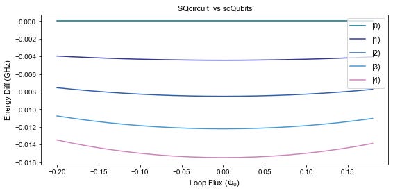
As we hoped, they seem to agree pretty well. For the lowest three energy states, the two simulation packages agree within 10 MHz. I think I’d prefer better agreement, but the scatter on your actually fabricated qubit frequencies will be much larger than 10 MHz (as of 2022).
Transmons: Takeaway
We undertook a simple split-junction transmon simulation for two reasons. The first is to start spec’ing out the components of our two-qubit device, and check that our choices for capacitance and critical current returned the expected frequency and anharmonicity. The second reason was to familiarize ourselves with the available superconducting quantum device simulation softwares. There was some initial confusion about results from the simulation packages, which has since been resolved (see footnotes prior to this). This experience does highlight how important it is to have correct intuition and deep understanding of what it is you’re doing, as well as team members that can sanity-check your work. Despite my near daily use of the transmon, I didn’t properly appreciate its characteristics in the ‘deep charging’ regime and thus failed to immediately identify which simulator was giving the unexpected result. Learn from my failures, I beg you.
The Coupler
The next major component of our two qubit device is the coupler. Without a coupling component, our two transmons won’t interact at all and will just be two individual, isolated qubits. We need couplers to do fun things like entangling two-qubit gates, the fidelities of which are a key metric in the current push for fault-tolerance.
Couplers can be quite simple (a humble capacitor) or quite complex with multiple SQUID loops, inductors, and capacitors. Fundamentally though, the coupler is parameterized by one property, the coupling strength, g, between two quantum oscillators (qubits, resonators, etc). This coupling strength is, by convention, normally written in cyclic frequency units, and is about half the rate of vacuum Rabi oscillations between two objects.
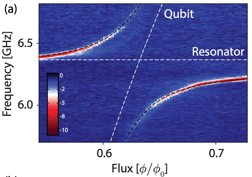
In actual experiments, we often measure g by observing the anti-crossing of two energy levels as they approach each other. The closer they are able to get, the weaker the coupling is. A coupling of zero would allow two coupled modes to cross without having any effect on each other. We are going to use our new simulation capabilities to predict g as a function of coupler and qubit parameters by simulating an anti-crossing between the qubits.
Capacitive
As an initial simple example we’ll start with a simple capacitive coupling between two copies of the transmons we’ve defined above. Our goal will be to get a sense of how g changes as a function of the capacitance, and whether it affects different energy levels differently. After that, we’ll take a look at more complex coupling schemes.

I used SQcircuit to do these simulations, correcting for the observed offset charge effects. Here’s the circuit definition:
init_flux1=0
init_flux2=0.4
C = 97 #fF
C_coup = 10 #fF
Ej = 24 #GHz
ng = 0.5
ncut = 30

sqcirc.set_unit_cap('fF')
sqcirc.set_unit_JJ('GHz')

loop1 = sqcirc.Loop(value=init_flux1)
loop2 = sqcirc.Loop(value=init_flux2)
C1 = sqcirc.Capacitor(value=C)
JJ1 = sqcirc.Junction(value=Ej/2, loops=[loop1])
JJ2 = sqcirc.Junction(value=Ej/2, loops=[loop1])

C2 = sqcirc.Capacitor(value=C)
JJ3 = sqcirc.Junction(value=Ej/2, loops=[loop2])
JJ4 = sqcirc.Junction(value=Ej/2, loops=[loop2])

C3 = sqcirc.Capacitor(value=C_coup)
elements1 = {(0,1): [C1,JJ1,JJ2],
             (1,2): [C3],
             (2,0): [C2,JJ3,JJ4]}


qubs = sqcirc.Circuit(elements1)
qubs.set_trunc_nums([ncut,ncut])
qubs.set_charge_offset(1,ng)
qubs.set_charge_offset(2,ng)
We define two identical transmons, coupled by a capacitor with 10 fF. Qubit2 is set to a flux bias of 0.4 Φ0, which brings its frequency down to about 3 GHz. This allows us to use qubit1’s flux bias to sweep its frequency through resonance with qubit2, hopefully demonstrating the anti-crossing. Let’s try it.

It is as we hoped! Closer inspection shows that g/2π ~145 MHz. Now we can go further and answer the next question: how does g change as a function of coupling capacitance? What happens when the transmons are weakly coupled with just 1 fF? What about with 50 fF?
We can re-run the simulation by rebuilding the circuit and changing the coupling capacitance only, then calculating the spectrum and extracting the value of g as above. Here’s the result:

Qualitatively, the result is as we would have expected. Bigger coupling capacitances yield bigger coupling values. Note that the relationship appears to be sub-linear, so there’s some diminishing returns to using huge capacitors to ensure large couplings between qubits9.
Inductive
You can repeat the exercise above using a static inductive coupling between the transmons, rather than a static capacitive coupling. The circuit would look something like this:

You may have legitimate reasons for desiring an inductive coupling, but note that numerically it is more difficult to simulate than the capacitive case. This is primarily because, inductive coupling requires that we have another node in the circuit, which means the Hamiltonian we’re diagonalizing is going to be larger, scaled by the truncation number (ncuts in scqubits). Adding nodes to your circuits will be expensive, so in general we like to choose our circuit elements and geometries to be able to minimize this when computational resources are scarce10.
I was intending to add a plot of two transmons with a static inductive coupler, but couldn’t make it work to my satisfaction. I think the amount of inductance you have to add to the transmons to get a decent coupling really loads down the modes and brings them too low, which probably necessitates bumping up the transmon junction Ic to compensate11. This is partly why I like static capacitive couplings. They’re way easier to implement and generally don’t mess up the qubits too much.
The Tunable Coupler
We’ve seen that we can couple two transmons together with either a static capacitive or static inductive coupling. We know that the strength of the coupling represents the frequency of photon (excitation) exchange between the two qubits, and it can be set by the magnitude of the capacitance or inductance used to achieve coupling.
The upside of this method is considerable simplicity in the design and fabrication process. The downside is that fabrication variations can cause some qubit pairs to be coupled much more strongly than other pairs, which can affect gate fidelities across the chip in question.
It is here that we come upon another trade-off. In exchange for additional complexity, more control lines, etc, you can create a tunable coupler that can provide a range of coupling strengths, including 0 (or as close to it as you get). On the other hand, to keep the simplicity of static coupling, you will run the risk of having wildly different realized coupling strengths due to fabrication differences between qubit pairs and couplers.
While I can’t make the decision for you, I can spend a few paragraphs describing the principles behind tunable coupling and demonstrate some of the more salient features using our handy quantum circuit simulators!
Tunable Inductive Coupling
One of the most common examples of tunable coupling between superconducting qubits is the tunable mutual inductance. The Google team had originally planned to use this kind of coupler in the quantum supremacy experiment, but later switched to a tunable capacitive coupling.
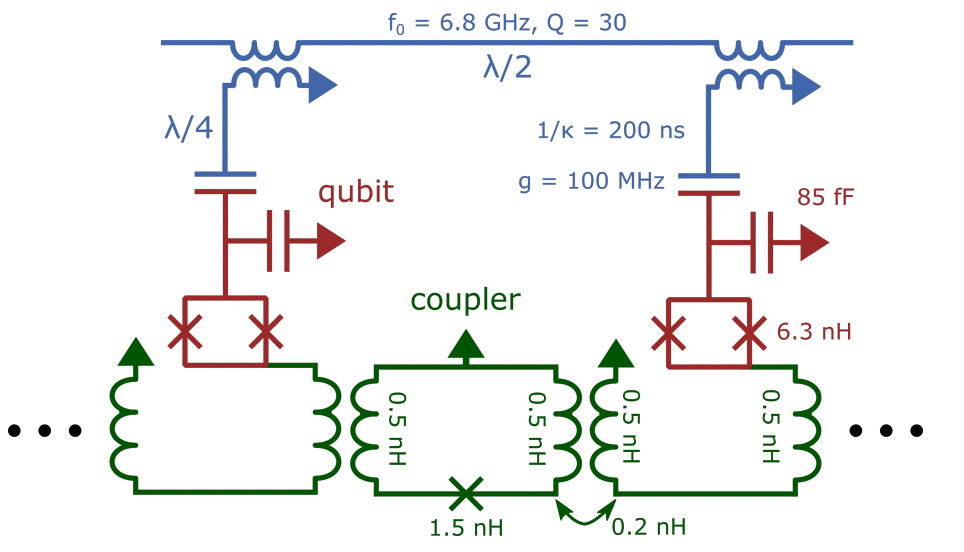
The coupler above has an implied current bias. You could also make the 1.5 nH junction into a DC SQUID so that we can use a flux bias instead of a current bias. In this case, we can turn ‘off’ the coupler by biasing it to Φ0/2. Physically this takes the inductance of the DC SQUID to infinity, which makes the 0.5 nH inductors the lowest impedance path that current can take, shunting it to ground and preventing coupling between the transmons.
I would love to show this to you, but our qubit simulator softwares don’t do mutual inductances, and transforming this into a galvanic coupling, rather than a geometric mutual would add more nodes to the circuit. Couplers in general are a rich subject, and perhaps I will write some posts dedicated to couplers themselves and how we can evaluate them without also necessarily simulating the qubits as well.
Tunable Capacitive Coupling
In the actual supremacy paper, the Google team mentions that they chose to move away from tunable inductive coupling and toward tunable capacitive coupling. While I didn’t see a circuit diagram, they do cite this paper from the Oliver group in their coupling discussion. Here’s the circuit diagram from the paper:
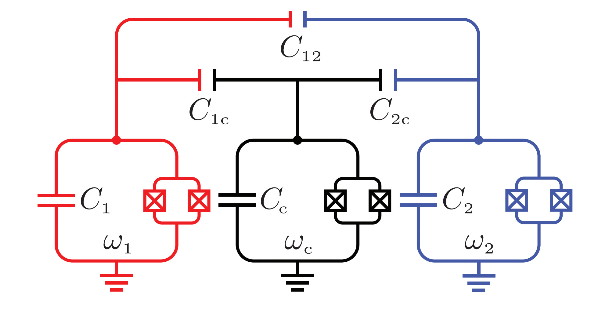
Red and blue are transmons which are capacitively coupled through another transmon (black). There’s also a (small) direct capacitance between the two main qubits (C12). If you read the paper, you’ll find that the explicit calculation of the coupling strength between the qubits as a function of the coupling-qubit’s frequency is quite involved.
In my original draft of this post, I had written a lengthy section here attempting to show this coupler should have an off-state just using classical impedances, but after a lot of angst and scribbling, I am convinced that this particular circuit doesn’t really lend itself to much of a handwavy, classical interpretation12. There is still a chance I just really messed up the algebra, which would be embarrassing, but I’m only human13.
I think this is largely because, as stated in the paper, the there are a bunch of interactions contributing to the off state in this coupler, both positive and negative coupling strengths that sort of cancel out at a certain flux bias. If you’re curious about why this works and you’re not willing to wait for my dedicated Coupler Post14, you’re going to have to read the paper.
OK so, maybe instead of doing all of this tiresome analysis, we can just numerically simulate a tunable capacitive coupling configuration and explore the parameter space in that way? Hell yeah we can!
Here’s the definition of the circuit I used in scqubits15:
tcap_coupled_tmon = """# transmon circuit
branches:
- ["JJ", 0, 1, 12,10]
- ["JJ", 1, 0, 12,10]
- ["C", 1, 0, 0.2]
- ["C", 1, 2, 4.84]
- ["JJ", 0, 2, 36,10]
- ["JJ", 2, 0, 36,10]
- ["C", 2, 0, 0.1]
- ["C", 2, 3, 4.84]
- ["JJ", 0, 3, 12,10]
- ["JJ", 3, 0, 12,10]
- ["C", 3, 0, 0.2]
"""
The parameters in the code block above correspond to our usual transmons defined at the very beginning at nodes 1 and 3. They are coupled to the coupler-qubit with C1 = C2 = 4 fF. Additionally, the coupler-qubit has shunt capacitance 200 fF as in the paper linked above, and Josephson junctions with Ic = 72 nA, each. I chose these coupler params to try to keep its eigen-modes above those of our qubits, as it makes me pretty uncomfortable to bring coupler modes down into the qubit band, but that’s just one of my hangups.
When constructed, external fluxes 1 and 3 control the transmons to be coupled, and external flux 2 controls the coupler itself. Note that I’ve also removed the small parasitic capacitance C12 as we are operating in the ‘ideal’ regime right now. In the future we will go back and add these parasitics to understand the true operation of the circuit.
I set the fluxes such that qubit 2 is sitting at 4.5 GHz, the coupler is at 0.3 flux bias, and we sweep qubit1 down through qubit 2 to observe the strength of the interaction.
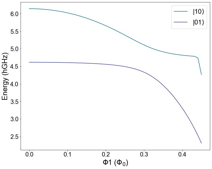
That seems legit to me, so the next step is to sweep the coupler flux bias while calculating the eigen-energies at each step. We can extract the coupling strength between the two qubits as a function of flux bias on the coupler and plot that. This will help us find when the coupler is off, as well as understand the range of interaction strengths available to the experimental team.
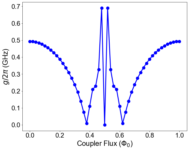
What do you think? Is it what you expected? This mostly closes with my expectation from the coupler, with one weird part being the very center point seemingly going to 0 coupling discontinously. That, combined with the strange kinks around 0.45 and 0.55, suggest to me that perhaps the coupler eigenmode is dropping into the region of interest (~4 GHz) and messing up my simple script that assumes the only two eigenmodes we encounter are those of qubit1 and qubit2. If you were doing this For Real, you’d make sure to understand and fix this problem before showing it to others.
One important feature I’d like to highlight is that region of 0 coupling at ~0.39 on the flux axis. That is the true ‘off’ position of the coupler. One major deficiency of basic tunable couplers is that the off state is not a local min or max on the curve. That means its very hard to really turn off qubit-qubit interactions, even in cases with vanishingly small capacitances between the qubits. 1/f flux noise on the coupler flux bias line will randomly turn the coupling on and off, which is likely to affect 2-qubit gate fidelities (not in a good way).
Concluding Thoughts
Since this post is already getting super long, I think it makes sense to wrap up here with some overall conclusions and then a list of the next steps you might take if you were serious about having this thing fabricated and tested.
Take aways
I tried to make this post an example of just going out and Doing the Thing instead of endlessly preparing yourself to Do the Thing. In this case, we wanted to use an open-source superconducting circuit simulation package to evaluate the operation of a tunable coupler between two qubits in service of our Open Source QPU design. We have only just scratched the surface of the power of these software packages. There is much more to learn.
Having a strong baseline knowledge of superconducting qubits16 is helpful to serve as an internal sanity check of results and to help identify software bugs.
The simulation packages themselves can help newcomers and seasoned professionals develop better intuitions for superconducting qubit properties, especially for unusual qubits.
Static couplings are easy to simulate, but can introduce risk in real-world environments due to fabrication variations.
Tunable couplings can help lower the risks inherent in static couplers, but come with their own issues. One of which is that the 0 coupling state is not at a noise-insensitive point of the coupler flux bias curve.
Next Steps
There are a few obvious next steps for continuing the design process. Here is what I would do, if I were responsible for this design in a real organization:
Resolve issues with the tunable coupler simulation (we think we know what’s wrong).
Use result of coupler simulations to do some 2-qubit gate simulations to determine whether acceptable gate fidelities are even theoretically achievable.
Begin physical layout and physical electromagnetic simulations to ensure that device sizes are not impractically big or small. i.e. Did you accidentally require that your coupling capacitors are below the minimum deposition width of your superconducting metal? Simulate expected mutual inductances, capacitances between parts, and determine parasitic inductance and capacitance values (ex: C12 from circuit schematic above).
Return to scqubits or SQcircuit and resimulate the whole device but with the parasitics this time. Do you still get acceptable performance? Are follow-up gate simulations required?
Continue iterating until the design ‘closes’ or it is shown to be impractical to achieve with current fab process.
Here’s the Quantum Supremacy paper and its Supplementary Materials.
The limit is of order 1/α. That is to say that microwave pulses shorter than 1/α in time will have some frequency components (spectral content) that exceed our anharmonicity, α, and can accidentally excite |2〉. The interested reader can prove this for themselves by Fourier transforming a Gaussian distribution and observing the results as the initial Gaussian is made fatter or thinner.
This is the first ‘deficiency’ I noticed with both of the circuit simulators in question. They natively use theorist units, not the units of actual circuit elements. SQcircuit does have the option to define capacitances in fF and inductances in pH or nH. Unfortunately, neither package lets you define Josephson junctions with their critical currents.
Junctions in parallel add Ic, so if you want a symmetric split junction transmon with the same parameters I defined above, you’ll want 2x 24 nA junctions.
Don’t forget to keep track of your implied Planck constants in this step.
Note that if you’re making a split-junction transmon explicitly using the YAML syntax, you’ll need to switch the node ordering on your junctions (see below) for the external flux variables to be correctly generated. This is a bug and this workaround is temporary. I’ve opened an issue.
tmon_yaml = """# transmon circuit
branches:
- ["JJ", 0, 1, EJ=12,10]
- ["JJ", 1, 0, EJ,10]
- ["C", 1, 0, EC=0.2]
"""An earlier draft of this post observed a mistake in how much offset charge was applied to SQcircuit transmons. This has since been resolved, but you can refer the github issue for more details.
As we’ll see in future installments, using huge capacitors comes with major trade-offs in physical design space, as well!
You could spin up an AWS instance, whatever that means, and just blast these simulations across a shitload of cores, but your humble author is working on a single laptop.
The motivated reader should try resolving this issue.
I really want there to be a classical microwave engineering explanation for this, but I ran out of patience trying to get it to work out.
Figure of speech. I’m really a floating, unblinking, sentient atom.
Technical posts take a long time. BUT if you’re a coupler expert and have a nice, intuitive derivation for why/how capacitive couplers work, post a comment! Or send me an email at quantumobserverblog (at) gmail (dot) com.
Note that I didn’t use any symbolic definitions in this particular circuit, due to an issue I had with over-burdening the symbolic matrix inversion. You can read through this issue for more details and an alternate work around if you want to use symbolic parameters.
This should not discourage novices, just note that it helps to have a more experienced friend around to help discuss ideas and results.
Also there’s a new tunable coupler paper that just dropped: https://arxiv.org/pdf/2207.06607.pdf
What if you made a coupler out of two transmons instead of one? Might be fun to simulate
Thanks a lot for the blog post! Really appreciate the side-by-side comparison of SQcircuit and scQubits. I totally agree with "Doing the Thing instead of endlessly preparing yourself to Do the Thing"!
To answer your question whether the tunable coupling vs. coupler flux curve is what I expected: No ;-) I would expect that at zero coupler flux, when the coupler is far removed from the qubits in frequency, so it doesn't participate much and the qubits are almost uncoupled. But at zero coupler flux, the plot shows a gap=2*coupling of 500 MHz which is super large.
After some digging: it looks like when you construct a circuit from YAML with scQubits, it uses a default cutoff of |n| = 5 for the non-periodic variables, which is of course too small to model transmons. If you make the cutoff much larger the calculation takes long, so hierarchical diagonalization is probably the way to go. Code below, this works with scqubits==3.0.2 :-)
The "leading order" intuitive explanation of tunable couplers I'm familiar corresponds to eq (2) in Yan et al, https://arxiv.org/abs/1803.09813. It says that a direct capacitance gives a positive coupling, and an indirect coupling via the coupler transmon gives a negative coupling. So if you get the indirect coupling just right by tuning the coupler frequency, the two coupling channels cancel out. I can't really back that explanation up, so I'm looking forward to your coupler blogpost!
That would suggest that the direct qubit-qubit capacitance is necessary to have an off-point. I.e., the stray qubit-qubit capacitance is a feature not a bug here. That turns out to be the case numerically: Plotting the coupling on a logscale, it never actually reaches zero, but stays above 1MHz or so which would be too large in practice. If you add a small capacitance between nodes 1 and 3, with a charging energy of say 48.4 GHz, there is a good off point. Let me know if you agree!
I agree with you that beyond a flux of 0.4 or so, the coupler goes below the qubits in frequency, so getting the coupling as the difference between the second and first excited energies no longer works.
```
import numpy as np
import scqubits as scqub
import matplotlib.pyplot as plt
tcap_coupled_tmon = """# transmon circuit
branches:
- ["JJ", 0, 1, 12,10]
- ["JJ", 1, 0, 12,10]
- ["C", 1, 0, 0.2]
- ["C", 1, 2, 4.84]
- ["JJ", 0, 2, 36,10]
- ["JJ", 2, 0, 36,10]
- ["C", 2, 0, 0.1]
- ["C", 2, 3, 4.84]
- ["JJ", 0, 3, 12,10]
- ["JJ", 3, 0, 12,10]
- ["C", 3, 0, 0.2]
"""
tcap_tmons = scqub.Circuit(tcap_coupled_tmon, from_file=False, ext_basis="discretized")
tcap_tmons.configure(transformation_matrix=np.eye(3), # work in node variables, rather than automatically choosing variables
system_hierarchy=[[1], [2], [3]], # hierarchical diagonalization, treat each node var as a subsystem
subsystem_trunc_dims=[7, 7, 7]) # diagonalize and truncate each subsystem to 7 dimensions before diagonalizing joint system
for i in [1, 2, 3]:
setattr(tcap_tmons, f'Φ{i}', 0.3) # Set both qubits at flux 0.3
setattr(tcap_tmons, f'cutoff_n_{i}', 50) # To diagonalize each subsystem, go up to |n|=50, rather than the default |n|=5
flux_array = np.linspace(0.0, .4, 201)
# flux_array = np.linspace(0.35, .37, 201) # Zoom in on the off point
fig, ax = tcap_tmons.plot_evals_vs_paramvals('Φ2', flux_array, evals_count=7, subtract_ground=True)
ax.set_title('Spectrum vs. coupler flux')
spec = tcap_tmons.get_spectrum_vs_paramvals('Φ2', flux_array, evals_count=3, subtract_ground=True)
gap = spec.energy_table[:, 2] - spec.energy_table[:, 1]
print(f'Minimum coupling [GHz]: {np.min(gap)/2=}')
plt.figure(figsize=(10, 8))
plt.plot(flux_array, gap / 2)
plt.xlabel('$\Phi$2 ($\Phi_0$)', fontsize=24)
plt.ylabel('Coupling (GHz)', fontsize=24)
plt.yscale('log')
plt.tick_params(labelsize=20)
plt.title('Coupling vs. coupler flux')
plt.tight_layout()
plt.show()
```