
Virtual Qubits and Quantum Machines, Pt. 1
In Which I Don't Understand


During my hiatus I’ve been reading a little bit about thermodynamics with quantum systems, virtual qubits, quantum machines (not the company) and so on. Unfortunately, due to being kind of dumb, I mostly read these papers slack jawed, occasionally muttering ‘what the fuck’ under my breath. If you were to look at my notes scribbled in the margins of these papers, you’d mostly see “????”, but the handwriting becomes more erratic deeper in the paper, betraying my increasing derangement.
That’s a lot of words to say I find some of this weird and confusing, so I thought I’d write up a post and maybe do some simulations.
The main trick that most of the papers I’ve read seem to rely on is the creation of a ‘Virtual Qubit’ with some arbitrary, engineered virtual temperature Tv. Here’s a sketch of how things usually go:
Define two qubits, A and B. You get to choose their energy levels.
Couple the qubits A and B to two different temperature baths with temperatures Ta and Tb1, allow them to thermalize (the qubits don’t interact, yet).
The temperatures and energy levels of the qubits define a 'Virtual Qubit’ with temperature Tv. This virtual qubit and its temperature is the key gimmick that enables some interesting downstream effects. The Virtual Qubit has energy spacing Eb - Ea.
Weakly couple a third qubit, C, with Ec = Eb - Ea to the virtual qubit.
If the temperature of qubit C, Tc, is greater than Tv, qubit C will cool. If Tc < Tv, qubit C will heat.
You can also do something interesting things like build an autonomous quantum clock using these kinds of systems.
It almost seems trivial, but I think the whole idea of the virtual qubit is kind of weird.
Starting with two qubits at different temperatures and energy levels is straight forward. We can let Eb > Ea in this case, and pretty easily write down the population distribution of each qubit.

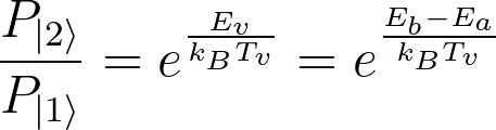
Thermal equilibrium at a given temperature lets us define a ratio between the ground and excited states:

This should be familiar to most people who’ve taken a Statistical Mechanics course, but it’s worth pointing out that the only way to get such a ratio > 1, requires negative temperatures. Instead of being extremely cold, like one might naively expect, negative temperatures are quite ‘hot’, in that they are required to achieve population inversion. this is a quirk of systems with discretized energy levels, rather than a continuum. If you are shocked and awed by this, I think any decent graduate-level stat mech book (Pathria?) should have an exercise that walks you through this derivation more systematically.
The same will be true of qubit B. The trick to getting a virtual qubit out of this is considering qubits A and B as a ‘composite’ system, in which two states will form our virtual qubit:


Knowing what we know about the temperatures and probability distributions of the component qubits, what can we say about the population and effective temperature of the virtual qubit?

By construction, the energy between the virtual qubit levels has to be the difference between Eb and Ea. Thus we’re left with an expression for the temperature of the virtual qubit:
For me, just looking at this equation is not particularly useful. The paper tells us that
“…the virtual temperature, as a function of the local energy level spacings Ea and Eb, can take a range of values, crucially all temperatures outside the range of Ta and Tb – it can be smaller or larger than both, and can even take negative values”.
I think something along the lines of ‘what. the. fuck.’ is an appropriate reaction here. It can take on any value outside of the range between Ta and Tb? Come on.
Let’s take a look:

This plot is totally unhinged. It’s so weird! Imagine telling someone that you can arrange two temperature baths in such a way that the temperature of a thing coupled to both is *checks notes* negative infinity. I slept through my Stat Mech class2, but even I know that's weird. Probably the people who are actually good at physics and make their living off of knowing statistical mechanics would tell you that this weird stuff happens because in these qubit systems you get to control the microstates (energy levels), which is just not true or feasible in classical systems. If any such experts are reading this and have a nice, intuitive explanation for why this makes sense, I would love to hear it.
Simulation- QuTIP
Sure we could ‘follow the math’ and end up with the result above, but what if we wanted to be dumb about it. Could we use numerical methods to get the same result?
To finish up this particular post, I’ll attempt to get the same result using a composite 2-qubit system simulated in QuTIP. The real good stuff would be to use a superconducting qubit simulator like scQubits or SQcircuit to see how this plays out under more realistic circumstances, rather than with ideal 2-state qubits. The sequel to this post will focus on implementing this in a device simulator and maybe trying to simulate some rudimentary quantum thermal machines.
Composite Hamiltonian
To start, I made a composite Hamiltonian3 in which the qubits share a ground state:
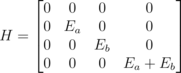
This is going to go into the QuTIP mesolve function to evolve some initial state to the final, thermalized state.
The other important thing we need to define are collapse operators4 which will to couple our system to the thermalizing bath(s). In the single qubit case, the collapse operator is an asymmetric Pauli x-operator. We know it has to be this way, because the thermal bath is causing bit flips in the qubit with excitation and decay rates that are related by the temperature of the bath and energy of the qubit.
It turns out the excitation and decay rates are related to each other in the same way as our probabilities5:

So to make a single-qubit collapse operator to represent thermalization with a bath at temperature T, we’d define a Qobj from the following matrix:

Since we’re impersonating theorists6 in this section, we will just normalize the decay rate to 1, so that the excitation rate will set the thermalization time for our system. It is not particularly difficult to extend the operator above to a system of arbitrary size (but it is annoying to type out). Extending it to our composite system will be left as an exercise for the reader7.
So if you set some reasonable initial state (I just use the ground state) and run mesolve to evolve the system in time you end up getting the following curves:

Which is basically what you’d expect. The final populations are defined by the interaction rates, which are themselves defined by the temperature of the bath(s). As above, I’ve set Ta = 50 mK, and Tb = 200 mK while Ea/Eb = 10. From our theory curve, we should expect a virtual qubit temperature of 300 mK.
Recall that the virtual qubit in this case is defined by states 1 and 2 in the composite system, so we will use the ratio of those steady-state populations to determine the virtual qubit temperature by solving this equation:
When I solve this using the results out of mesolve I get a virtual temperature 301.1 mK. Hooray!
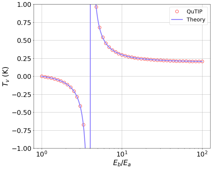
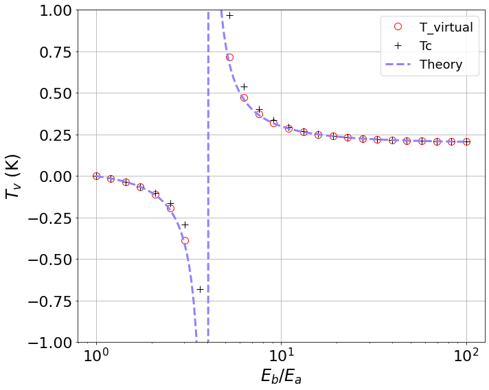
That’s just one point in parameter space. What about the rest?

Well. Ok. It’s not terrible. Better than I expected, really. For small ratios between the two physical qubit energies, the numerical and analytic approaches agree (red circles on top of the solid curve). We can reproduce both the negative temperatures and the elevated positive temperatures, but around Eb/Ea ~ 20 our numerical result begins to diverge from the desired asymptotic value. Why?
To be honest, I am not entirely sure, but I think it has something to do with the qubit energy levels vs thermal energy (kT). To illustrate what I mean, here’s the same plot, but instead of Ea = 1, I set Ea = 0.1, but the temperatures stay the same.
If you then scale down the temperature by 10x, you get the plot above this one, where the calculated temperatures diverge from the expected theoretical value for Eb/Ea > 20.
It would be interesting to return to this problem and fix it, but I’ve been working on this post for about 3 weeks now and, as they say, ‘perfect is the enemy of done’. So, since we've found a regime where the numerical result works across a wide range of Eb/Ea values, I will declare that we can move on for now8.
Heating a Qubit
The last part of this involves coupling a third qubit, Qubit C, to the system I described above. Necessarily, this third qubit is on resonance with our virtual qubit, and has its own temperature bath. Some interaction energy, g, is defined between the virtual qubit and Qubit C. It is supposed to be a ‘weak’ interaction, but I’m not sure relative to what. I did find that it actually needs to be strong compared to the environmental coupling that Qubit C experiences. That is to say, the virtual qubit must become the dominant part of Qubit C’s environment, otherwise we won’t be able to actually hit the virtual qubit temperature. Similarly, if Qubit C is not exactly resonant with the virtual qubit, the result of the heating/cooling will be worse than ideal9.
Thankfully, doing this in QuTIP just isn’t very hard, as you can see in the scripts I will link to at the end of this post10. In the plots above, we could select almost any temperature we want, outside of the range between Ta and Tb. If we just choose the parameters we've been using thus far: Eb/Ea = 10, Ta = 50 mK, Tb = 200 mK, then we would expect the virtual qubit to sit at 300 mK, which is what Qubit C should see. Interestingly, I only get the 300 mK when no collapse operators are supplied for Qubit C.
Let’s just reproduce the same plot we’ve been making throughout this post.
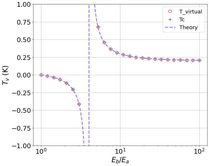
Very nice. Much agreement. Wow.
This is with no temperature bath for Qubit C outside of the virtual qubit. Now let’s pretend Qubit C is also at 50 mK, but has much slower decay/excitation rates than Qubit A and B. We can justify this by imagining that Qubit A and Qubit B were specifically made to be shitty and highly coupled to their temperature baths, but Qubit C is quite high-quality and is coupled as weakly as possible to its environment.
Hey, that’s not so bad! I'm a little bit surprised the temperature is over-estimated on the right side of the discontinuity, but perhaps that is a bug somewhere in the code. This result required that Qubit C decay/excitation rates into its environment were substantially slower (at least 1000x) than the Qubit A and B rates, which I think is achievable with current qubit design and fabrication knowledge.
Summary
Using the virtual qubit formalism, we’ve numerically and analytically shown that it’s possible to use two qubits with two different temperatures to manipulate the steady state of a third qubit, up to and including inducing a population inversion in the third qubit.
Along the way we’ve noticed some idiosyncracies of the numerical approach, as well as hints of ways in which this scheme could break down. It seems to work reasonably well with ideal qubits, perhaps you can use ideal qubits to build quantum thermal machines.
What do we get if we try this with, say, transmon qubits? Since we are not capitalist fat-cats and don’t have our own superconducting QC startups, we will have to restrict our investigation of this question to the realm of numerics. In the next installment, we’ll try using one of the superconducting circuit Hamiltonian solvers to tackle this problem. Stay tuned!
Appendix A- Code and Further Exploration
Here is a link to the scripts I used to make the plots in this post.
As you can see, the code is very primitive. You might be thinking to yourself, “what idiot wrote this? I could do it way better!” I encourage you to act on these feelings and prove to yourself that you can.
You’ll also notice that I didn’t really go beyond exploring some very basic features of these systems, but there is a rich array of changes to make! You may have noticed that our simplest composite system has six pairs of energy levels (4 choose 2), which means that you could define some other virtual qubits with different temperatures. Why not couple a 3rd qubit to those?
You may have many more questions after reading this post. Why don’t you take a crack at answering them for yourself?
In general, we let Eb > Ea, which also implies that Tb should be > Ta if you want to see the weird stuff.
In my defense, I would get extremely tired around 2-3 PM, which happened to be Stat Mech time. Much later I figured out a short (20 minute) nap right before would have fixed all of this. That’s my pro-tip for you.
The code I include in the appendix will actually have two ways of doing this. You can write down the diagonalized Hamiltonian directly, along with the collapse operators, or you can write the Hamiltonian as the tensor product of two single qubit Hamiltonians. Similarly, the collapse operator becomes the tensor product of single-qubit collapse operators. I like the tensor product approach because it means you only have to understand single-qubit physics, but can still generate composite systems and evolve them in time.
If you’re unfamiliar with this, the linked QuTIP documentation is a reasonable intro with plenty of links to further reading.
This is usually justified by an appeal to detailed balance in steady-state.
You’ll note in the code that I fail to truly commit to Full Theory Mode and set h = kB = 1. This is because I fundamentally don’t trust theorists (no offense) and I need the units to be there to act as a reliable way to catch errors.
Because I’m not a total monster, I will offer a clue. The collapse operator above will take the state 0 → 1 at the excitation rate (\Gamma_\uparrow), and state 1 → 0 at the decay rate (\Gamma_\downarrow). When you add more levels to your Hamiltonian, you need to arrange the operator to properly excite and decay the higher levels. This is much easier if you constructed your Hamiltonian as a tensor product of single-qubit Hamiltonians.
This is an important part of Professional Physics. Having a good sense for what needs to be resolved Right Now and what can wait until later could save you a lot of trouble. Of course, there’s always the lurking danger that you’re wrong about what is important, but that’s what keeps the job spicy and fun.
The end of this post has some links to scripts I wrote to make these plots, so you can use them as a jumping off point to tweak all kinds of parameters and observe the result.
Yes, yes, I code like a deranged criminal. Don’t at me.
I'm way more dumb, I'm still waiting for someone to explain topological qubits by Microsoft, in plain english.