

It has been noted that, on occasion, physicists like measuring things1. Measurements are great, but there’s one thing that makes them really wonderful, and that’s an uncertainty estimate. There’s nothing quite like really nailing the error bars properly.
Those of us in superconductive quantum computing like to keep our chips cold. Dilution refrigerators can routinely get our chips down to a crisp 20 mK2. Although, those temperatures are usually measured at the mixing chamber, not at the site of the qubits themselves. So how can we be sure that the qubits are properly thermalized at the base temperature of the fridge? That is to say, how can we be sure that the qubits see a 20 mK thermal environment and not something much hotter?
One might suggest that we use the same thermometer that tells us about the mixing chamber temperature. These Ruthenium Oxide (RuOx) resistors are capable of measuring down to a few mK, but the problem is their size. While small compared to the usual scales of human life, the fact that they are deposited onto chips roughly 1mm on a side means they are far, far too large to be incorporated into (contemporary) qubit chips3.
So what to do?
One natural approach is to just use the qubits themselves as thermometers! We can use the equation for the population of a given qubit energy level from our previous discussion of Virtual Qubits as a probe of temperature.
In principle, anything that changes with temperature is a thermometer, if you’re brave enough to use it. In our case, we can see that the qubit state populations change with temperature! The really great news is that researchers in the field have expended prodigious brainsweat getting quite good at figuring out what the qubit population is, at least of the lowest energy levels. This information happens to be generally useful for doing computations or something. The simplest expression is for that of the ground state:
So, as long as we can measure the occupation of the qubit ground state, we can figure out the temperature of the qubit. Hooray!
Mission Accomplished?
Regretfully, it’s not all backslaps and high fives, because there are more questions to be answered. For example, how good are qubits at being thermometers? What’s the limit on their signal to noise ratios? Is measuring energy eigenstate occupations the best way to get at temperature, or is there a different quantity that might be more sensitive?
In general, it seems like these questions have already been answered, so all we have to do is a little digging through Wikipedia and Google Scholar.
<10 Hours Later>
OK so there’s good news and bad news.
Good: There’s a paper that addresses directly this! Thermometry in the Quantum Regime: Recent Theoretical Progress4. Although we might be mostly concerned with qubits, this is a general problem. A quantum system with some energy spectrum can be used to measure temperatures. The paper has lots of interesting bits, some of which we’ll get to eventually. The short answer to the questions above is that we need to calculate the Quantum Cramer-Rao bound for our quantum system of choice. If you want to be reductive about it, that’s kind of it.
Bad: The paper is 58 pages.
Thermometry in the Quantum Regime
The authors prove fairly early on that the Hamiltonian is the optimal operator to be measuring (i.e. measuring the energy of the system minimizes the temperature variance). They go on to construct the optimal energy spectrum for temperature measurements (it’s degenerate) and then explore steady-state, non-equilibrium, and dynamical situations.
We’ll get back to those later, but first, as is tradition, we will make a detour into the classical realm to tackle the first problem.
Back to Classical
What the fuck is the Cramer-Rao bound? And more importantly, how to calculate it?
I found this paper: Cramer-Rao Lower Bound and Information Geometry by Frank Nielsen5 paper through a Twitter mutual and it proved to be quite useful. I recommend reading through section 2.2.
An earlier version of this post had a lengthy recap of that information geometry paper, but I can’t really do it justice, nor do I have a more intuitive way of explaining/thinking about it, yet. So instead, I quote the relevant part of the paper6:
Suppose the regularity conditions state above hold. Then the variance of any unbiased estimator of θ, based on an independent and identically distributed (IID) random sample of size n, is bounded below by 1/(n*I(θ)), where I(θ) denotes the Fisher information in a single observation, defined7 as
\(I(\theta) = -E_\theta \left[ \frac{d^2l(x;\theta)}{d\theta^2}\right] = \int -\frac{d^2l(x;\theta)}{d\theta^2} p_\theta (x) dx\)
E is the expectation value, and the function l(x;θ) is the log of the likelihood function of our probability distribution, p(x;θ).
What to make of this ‘Fisher Information’?8 Well if you recall your training, you’ll note that the value is strongly dependent on the curvature (2nd derivative) of the log-likelihood function. If the log-likelihood is flat or has broad peaks, the Fisher information will necessarily be small, so the lower bound on the variance of the estimator must be large. Conversely, if the log-likelihood is strongly peaked, then the Fisher Information will be large, leading to a small lower bound on the variance of the estimator.
With that in mind, we can just go ahead and calculate a few Fisher informations to get a feel for what we’re working with. If you don’t feel like coding this up on your own, you can use my python notebook9.
Analytic Approach
Recall that we are using the Gibbs distribution as our probability.
Do we need to take the natural log of this? We COULD, yeah, but let’s not rush into anything to hastily. Can we do something more smooth-brained that might still be useful? Originally I had thought it would be trivial to just approximate this as a harmonic oscillator and take some derivatives, ending up with an analytic expression. And, indeed, if you work in inverse temperature terms, β = 1/kT, and take all of the derivatives w.r.t. β, then the math is quite simple. BUT, as far as I can tell, that answer is wrong, because the temperature knob is the the thing we care about. I think you end up having to convert your derivative back to temperature terms, which is kind of a pain10.
Instead, since compute is abundant and practically free, we’ll just calculate these things directly!
Toy Models - TLS
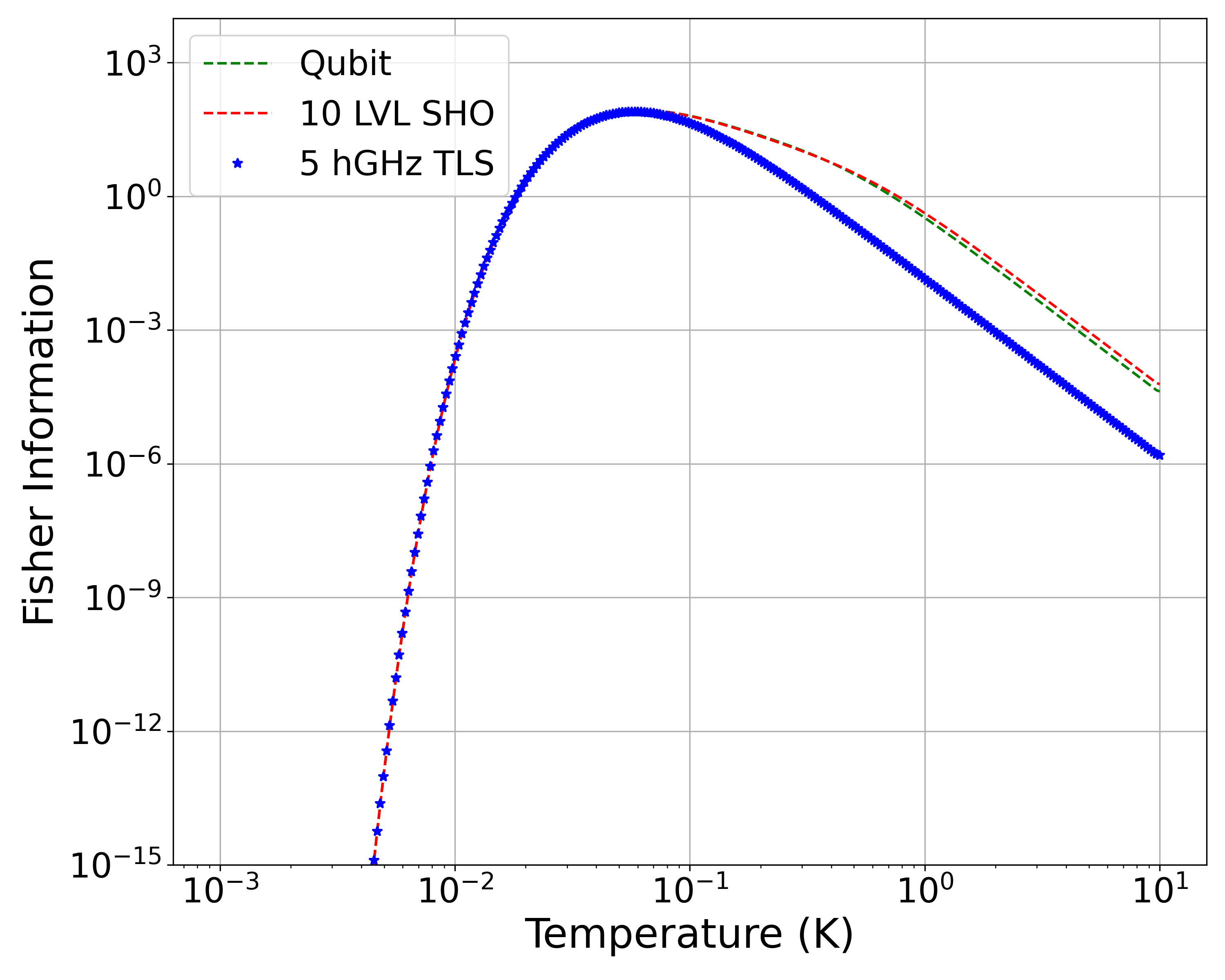
I start with the smallest, system I can think of: the two level system. In fact, I’ll plot ten Fisher information curves of TLS with energy gaps ranging from 1 - 10 hGHz.


While the Fisher information plots and temperature uncertainty plots look quite different between the TLS we simulate here, the minimum of the relative temperature uncertainty turns out to be exactly the same for each system11! I think this is reasonable, because why would changing the energy gap change the relative sensitivity of the system (at the optimal temperature)?
After simulating a bunch of different systems, I’ve concluded that, while the Fisher Information is a nice plot to look at, fundamentally the relative temperature uncertainty is the more important plot. I will keep those in what follows, and omit the plots of the absolute temperature uncertainty.
Toy Models - Resonators
The next thing I decided to do was compare the 1 hGHz TLS behavior to the first 10 and first 100 states of a resonator with fundamental frequency 1 GHz. This is just a comparison to a simple harmonic oscillator.

From the Fisher Information, we can see that both SHO implementations (10 states and 100 states) have a taller and wider peak than the TLS. I attribute this to the additional available states that can provide temperature information. We can also see a tiiiiiny divergence between the 10 and 100 level SHOs (red and green traces) out above 100 mK. We actually should look at this plot in log-log scale to appreciate the differences between the 10 and 100 level SHOs.

Much better! Now we can take a look at the relative temperature uncertainty. From the FI plot, we should expect the best performance from the 100 level SHO.

As expected the 100 level SHO has a wider range of better temperature sensitivity than either the 10 level SHO or the TLS. Note that these plots are all single-shot results. Still, it’s interesting and amusing to see that the relative temperature uncertainty is quite bad, even for the 100 level SHO! Since the temperature uncertainty is inversely proportional to the square root of the number of samples, simply taking 100 shots would get even the TLS below 100% relative uncertainty.
Toy Models - Qubits
Next thing I did was crack open scQubits to create a transmon energy 5 GHz and anharmonicity -100 MHz. I grabbed the first 10 eigenstates of that transmon and compared to a 5 hGHz TLS and a 5 GHz ‘resonator’. It’s important to note here that, if I wanted to do this strictly correctly, I should use the Quantum Cramer-Rao bound, which relies on the Quantum Fisher Information.
We will return to this later. For now, let’s just see what our, uh, quasi-classical12 approach tells us about qubits vs TLS vs SHO.

This seems to basically make sense. Transmons are weakly anharmonic, so they’re very similar to resonators. The difference is just enough to make them usable as qubits, but clearly not enough to improve their thermometry performance13.
The last thing I want to do here is conjure up the system that the authors of the paper I linked above claim is optimal: the n-fold degenerate TLS. Here’s Figure 1 from their paper, explaining the idea:
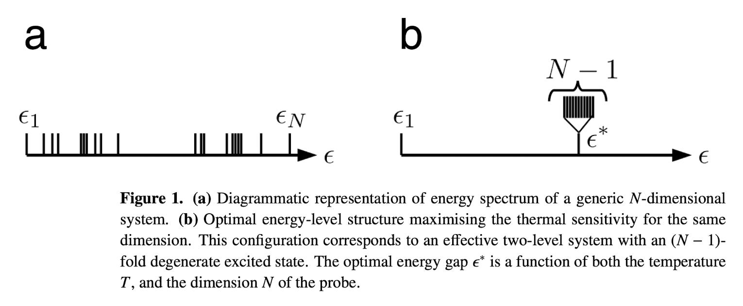
So I will make a system with 10x degeneracy at 5 hGHz and see where that gets us.

Well, that certainly seems to perform better at the optimal temperature. Remember, this is still ‘single-shot’.
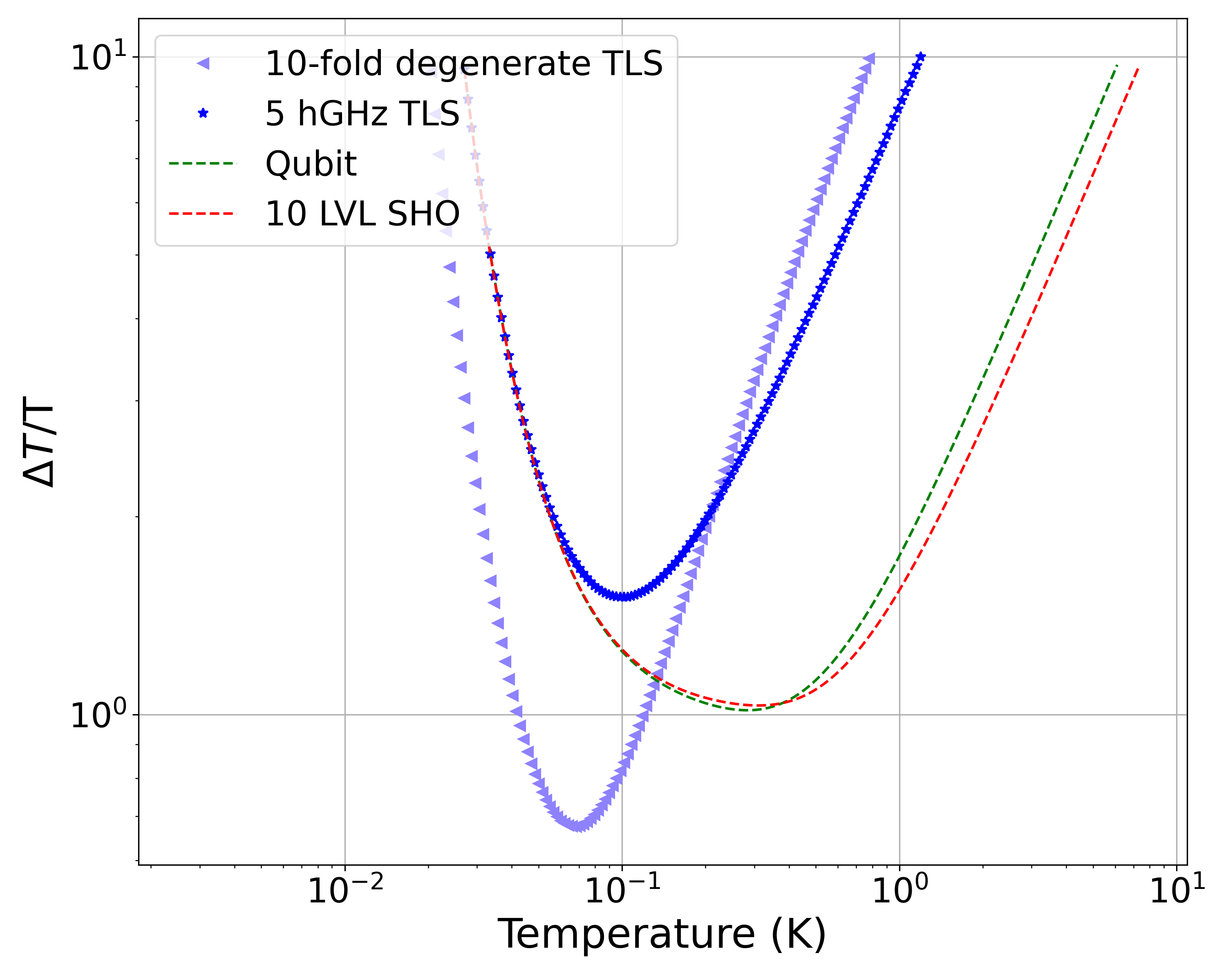
It looks like this thing has roughly sqrt(10) times better optimal relative uncertainty, compared to the standard, non-degenerate TLS. It also has much better lower temperature performance than any of the other systems, at the cost of its high temperature performance.
In terms of operating range, it seems like we can get most of a decade of decent performance out of either the qubit or the SHO, as long as we take multiple samples.
Conclusions and Open Questions
The ‘quasi-classical’ approach has quantum thermometers looking kind of shitty! The Lakeshore RuOx spec sheet quotes +/- 1 mK uncertainty at 10 mK14. One thing I’ll point out is that I think the performance of the resonator & qubit systems is a little misleading, because we rarely actually measure beyond the second or third excited state, so we end up throwing away some information. Since we prefer to pretend that superconducting qubits are two-level systems, it is likely the case that the true relative temperature uncertainty for the transmon we simulated here is simply very close to the ideal TLS.
I found that dipping a toe into a little bit of statistical formalism was far more interesting than I had expected. Once I expunged my many code bugs15, the simulations started going much more smoothly. Thanks to modern computing power, it’s pretty easy to numerical estimate the Fisher-Information (and Cramer-Rao bound) of some arbitrary arrangements of energy levels. We took the easy way out, but in the pieces that follow, I think it would be fruitful to compare quantum calculations with what we did here.
I’m interested in answering some subset of the following questions:
Will the quantum Cramer-Rao implementation for single qubit/resonator systems give us essentially the same performance as this quasi-classical approach?
What aspects of quantumness will provide the greatest benefit? Will this just be a case of ‘moar entanglement gud’?
Will we continue to conclude that highly degenerate systems are ‘optimal’?
What would we consider optimal? How can we engineer that?
What does, say, an Ising spin chain look like as a thermometer?
What about other quantum systems that we don’t usually think of as having energy levels (CBT or NIS thermometers)?
Is all of this calculating and simulating pointless when we begin to consider the entire system of readout and the noise introduced there?
What is the C-R bound for a RuOx thermometer?
Citation needed.
For the theorists among you, this is about 420 hMHz.
Not to mention that we generally frown upon putting normal, non-superconducting metals near our qubits.
arXiv link: https://arxiv.org/abs/1811.03988
If you spend enough time mucking about in this world, you come to the realization that everything is Information Theory is Geometry is Thermodynamics. This is pretty cool, but also bad for me because I sucked at geometry in school.
I had to paraphrase a little because substack doesn’t allow inline LaTeX.
The most general definition is that the Fisher Information is the mean of the square of the score (the first derivative of the log-likelihood). In some cases it can be written as the negative derivative of the score.
Gavin Crooks wrote an elegant note on Fisher information that I found useful. You can find it here: Fisher Information and Statistical Mechanics.
As usual, I make no guarantees, excuses, or apologies with respect to the quality of the code.
And a lot more LaTeX than I want to using Substacks ok-ish UI.
Just shifted over in temperature depending on the energy gap.
Whenever I see ‘quasi-classical’ I always take it to mean “I was too scared/lazy to use actual quantum mechanics”.
When treated in this strange way.
RX-102B-RS
Pro-tip: you should always be explicitly defining your sample spacing when using `numpy.gradient`.
Damn I do like your writing style. When I read your work I feel like someone's talking to me and I'm just basking in it. Amazing job as always.